1-Nearest Neighbor Prototypes
Selecting prototypes that best represent the entire dataset without compromising 1-Nearest Neighbor model performance. This experiment compares random selection versus label-based clustering selection on the MNIST dataset.
Brief Introduction
Our goal is to select prototypes that best represent the entire dataset without compromising a simple 1-Nearest Neighbor model performance. This is an effort to reduce the high storage and computing requirements in real-world settings. The two selection processes that I experiment with are random selection and label-based clustering selection.
The random selection process is uniformly selecting a smaller subset of the training data at random and is used to carry out the 1-Nearest Neighbors classification task. It would make more sense to obtain a richer subset of the data if we take advantage of the labeling. The label-based clustering selection process accumulates subsets of the data under each of the labels by finding where the data is most dense.
To find where the data is most dense under each of the labels, we can carry out a KMeans routine to find these data points and 'throw away' the data that is 'noisy' (e.g. far away from the clusters). If we do this for each of the labels respectively, we can combine all the cluster centers for each of the labels found by KMeans, and call those our prototypes.
To carry out this idea I use sklearn.cluster.MiniBatchKMeans for clustering
and sklearn.neighbors.KNeighborsClassifier to carry out the 1-Nearest Neighbor
classification task.
Diving into Code
import seaborn
import numpy as np
import matplotlib.pyplot as plt
from sklearn.neighbors import KNeighborsClassifier
from sklearn.cluster import MiniBatchKMeans

from mnist import MNIST

% matplotlib inline
% config InlineBackend.figure_format='retina'
I use the classical MNIST multi-class classification task (i.e. classify a handwritten digit to 0-9). Using python-mnist we can easily import our training and testing data.
# data loader
mndata = MNIST('./python-mnist/data/')

X_train, y_train = mndata.load_training()
X_test, y_test = mndata.load_testing()

# convert into numpy objects
X_train, y_train = np.array(X_train), np.array(y_train)
X_test, y_test = np.array(X_test), np.array(y_test)

print("training set size: {}\\ntesting set size: {}".format(X_train.shape, X_test.shape))
training set size: (60000, 784)
testing set size: (10000, 784)
There's exactly \(60,000\) and \(10,000\) data points in the training and testing sets respectively. The data (handwritten digits) lie in a high dimensional space which will be a huge bottleneck for carrying out a classification task in a production environment since for any query data point we have to compute pair-wise distances to each and every other data point in the training set. This becomes a much bigger problem as the size of the training set increases. This drawback motivates our search for prototypes! We want to reduce computation time while still maintaining model performance.
Below is the simple prototype selector that will get us random and label-based prototypes from the data. An instance of this class will get us a subset of size \(M\).
class PrototypeSelector:
    """
    X: training data set
    y: training labels
    return: prototype set of size M
    """

    def __init__(self, X, y):
        self.X = X
        self.y = y

    def get_prototypes(self, method, M):
        """
        method: the method to get prototypes
        M     : number of prototypes to return (size of subset)
        """
        if  method == 'random':
            indicies = np.random.permutation(self.X.shape[0])[0:M]
            return self.X[indicies,:], self.y[indicies]

        if method == 'label-based':

            x_samples, y_samples = [], []
            for class_ in range(num_classes):
                indicies = [i for i,val in enumerate(1*self.y == class_) if val == 1]
                k_means = MiniBatchKMeans(n_clusters = int(M/10)).fit(self.X[indicies])

                x_samples.append(k_means.cluster_centers_) # use cluster centers as prototypes
                y_samples.append(self.y[indicies][0:int(M/10)])

        return np.concatenate(x_samples), np.concatenate(y_samples)
Crucial to the experiment is the parameter \(M\), this denotes the size of the subset that will be returned through the selection process. Later in the experimentation we'll tinker with this parameter and get a sense of model performance under different subset sizes \(M\). Ideally, we'd want to have the smallest size \(M\) such that model performance is still 'reasonable'.
Random Selection
The random selection process is very simple: given a set of data points \(X\), the
PrototypeSelector will randomly permute the data set and return the first
\(M\) instances.
Label-based Selection
In short, the label-based selection method accumulates KMeans cluster centers (i.e. the prototypes) under each of the labels such that the total number of cluster centers found in each label is given by
$$ \frac{M}{\text{# of labels}} $$
If we find cluster centers independently for each of the labels (i.e. there are ten digits
0-9), we will have a prototype set of size \(M\), because we would have
accumulated \(\frac{M}{\text{# of labels}}\) for each. We are essentially finding the same
amount of prototypes under each of the labels to add into the final prototype set such that
it has size \(M\).
The label-based method can be summarized by the following steps:
- For each label \(i\) find the data corresponding to that label: \(X_{i}\).
- Execute
KMeansroutine with the number of clusters set to \(\frac{M}{10}\) on the data \(X_{i}\) - Accumulate these cluster centers as the prototypes
After accumulating the prototypes under each label, we should have a much better representation of prototypes of the training data of size \(M\). This method chooses prototypes where the data is most dense (i.e. cluster centers) and essentially removes uninformative noise in the data set that just adds an extra layer of computational overhead to carry out a classification task.
Experiment
Again, our goal is to find the smallest (or as small as we can) subset of the training data such that we don't compromise the model performance of 1-nearest-neighbors classifier. In short the nearest neighbor classifier finds the label of the closest data point to a query data point and sets its prediction to that label.
The MNIST data set has \(60,000\) data points living in \(784\)-dimensional space. Like I
mentioned earlier, we want to have a training set that is as small as we can so I experiment
with subsets of size \(M = 1000, 5000, 10000\). This parameter controls the size of the
subsets returned by PrototypeSelector.
num_iter = 5
num_classes = 10
M_vals = [1000, 5000, 10000]
With the help of some helper functions we can get the accuracies and error bounds of the 1-nearest neighbor predictions.
def accuracy(y, y_pred):
    '''
    y : actual labels
    y_pred: predicted labels
    return: accuracy of model (%)
    '''
    return np.sum(1*(y_pred == y))/len(y)

def get_error_bounds(accuracies):
    '''
    accuracies: list of accuracies of model over n trials
    return: error bounds on the accuracies
    '''
    n = len(accuracies)
    t = 2.776 # 95 percent confidence interval
    mean, sigma = np.mean(accuracies), np.std(accuracies)
    bound_1 = mean + t*sigma/np.sqrt(n)
    bound_2 = mean - t*sigma/np.sqrt(n)

    return abs(bound_1 - bound_2)
Because of the random nature of this experiment, the number of iterations (num_iter)
of each experiment is set to 5, so we can obtain a confidence interval on the accuracies of
the model based on different subsets of size \(M\) and different selection methods. We can
get the error bounds using the get_error_bounds function and passing it a
sample of model accuracies.
Also after conducting num_iter on each configuration we can get a \(95\%\)
confidence interval on the accuracies of the model using the formula:
$$ \bar{X} \pm t\frac{s}{\sqrt{n}} $$
Where \(\bar{X}\) is the sample mean, \(s\) is the sample standard deviation, and \(n\) is the number of trials. The \(t\) score for a problem with \(n - 1 = 4\) degrees of freedom and level of significance \(\alpha=0.025\) is given by \(t = 2.776\).
Running the Experiment
# error bound collector for prototype selection
random_errs_collector = []
label_based_errs_collector = []

random_accs_collector = []
label_based_accs_collector = []
selector = PrototypeSelector(X_train, y_train)
for M in M_vals:

    random_accuracies, label_based_accuracies = [], []
    for iteration in range(num_iter):

        # uniformly random selected subset
        X_rand, y_rand = selector.get_prototypes('random', M)
        random_model   = KNeighborsClassifier(n_neighbors=1).fit(X_rand, y_rand)
        y_pred         = random_model.predict(X_test)
        random_accuracies.append(accuracy(y_test, y_pred))


        # label-based selection
        X_label_based, y_label_based  = selector.get_prototypes('label-based', M)
        prototype_model = KNeighborsClassifier(n_neighbors=1).fit(X_label_based, y_label_based)
        y_pred          = prototype_model.predict(X_test)
        label_based_accuracies.append(accuracy(y_test, y_pred))

    # get confidence intervals errors on accuracy
    random_errs_collector.append(get_error_bounds(random_accuracies))
    label_based_errs_collector.append(get_error_bounds(label_based_accuracies))

    # average accuracy over trials for each M
    random_accs_collector.append(np.mean(random_accuracies))
    label_based_accs_collector.append(np.mean(label_based_accuracies))
Results
Now we have access to the results of the experiment! Particularly, we have the accuracies and error bounds of each prototype selection method (random and label-based) under different configurations of \(M\) (sizes of prototype subset) for a 1-nearest neighbor classifier.
My gut feeling tells me that a uniformly random selection of training data will not outperform the label-based selection method because we are choosing subsets that are highly representative of the data with respect to the classification task. First let's get a baseline accuracy on the complete training set.
Baseline with Full Training Set
The 1-nearest neighbor results using the full training set is used as a baseline for comparison in model performances from full and prototype training sets.
full_set_accs, full_set_errs = [], []
for i in range(num_iter):
    full_model     = KNeighborsClassifier(n_neighbors=1).fit(X_train, y_train)
    y_pred         = full_model.predict(X_test)
    curr_accuracy  = accuracy(y_test, y_pred)
    full_set_accs.append(curr_accuracy)

full_avg_acc = np.mean(full_set_accs)
>>> full_avg_acc
0.9690999999999999
Running 1-nearest neighbor on the complete data was very computationally heavy and took
significantly longer than the experiments themselves. The final average
accuracy on the complete training set: full_avg_acc = 0.9691
Visualization
The plot below summarizes the results of our experiments:
plt.figure(figsize=(10,10))
plt.plot(M_vals, random_accs_collector, 'g-o', label='Random Selection')
plt.plot(M_vals, label_based_accs_collector, 'r-o', label='Label-Based Selection')
plt.axhline(y=full_avg_acc, color='b', linestyle='--', label='Full Dataset Baseline')
plt.title('Prototype Selection Performance', fontsize=20)
plt.xlabel('Number of Prototypes (M)', fontsize=15)
plt.ylabel('Accuracy', fontsize=15)
plt.xticks(M_vals, fontsize=12)
plt.yticks(fontsize=12)
plt.grid(True, alpha=0.3)
plt.legend(fontsize=12)
plt.tight_layout()
plt.show()
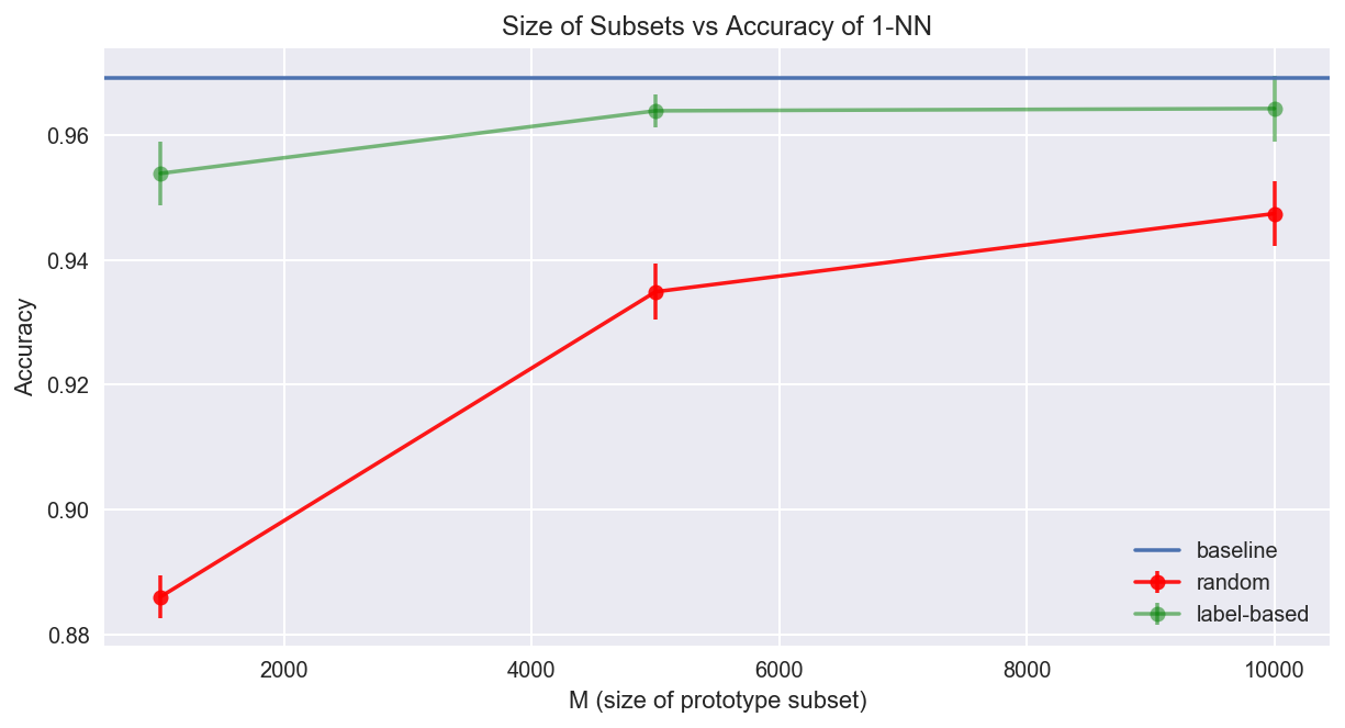
Conclusion
The experiment demonstrates that label-based clustering selection provides a much richer set of prototypes compared to random selection. By using KMeans to find cluster centers under each label, we effectively capture the density of the data while removing noisy outliers. This approach maintains model performance while significantly reducing the computational requirements of 1-Nearest Neighbor classification.
The results show that even with a significantly smaller subset of the training data (e.g., \(M = 10000\) compared to the full \(60000\) examples), the label-based approach can achieve comparable accuracy to using the complete dataset, while drastically reducing storage and computation time.