March 2019 · ·

Coordinate Descent for Logistic Regression

A walk-through of two coordinate descent variants on cross-entropy loss for a binary UCI wine task, compared against scikit-learn's logistic regression baseline. Coordinate descent is a fundamental optimization tool in machine learning because it scales to high-dimensional problems, lets us update one parameter at a time, and underpins many modern large-scale training routines.

Introduction

This post showcases two different approaches to implementing coordinate descent on a model defined with cross-entropy loss. Coordinate descent can struggle with non-smooth multivariate functions, as the algorithm may get stuck at non-stationary points where level curves are not smooth. However, it has gained significant interest for large-scale problems, where it has proven competitive with other algorithms for training support vector machines and performing non-negative matrix factorization.

In this experiment I implement coordinate descent using the following approaches:

Randomly optimize along a random coordinate
Optimize along coordinate with the largest gradient in magnitude

To benchmark the solutions I implemented a standard logistic regression model without focusing on validation and was just used to obtain scikit-learn's implementation of gradient descent and final loss. The model is trained with the wine.data dataset provided by UCI machine learning repository.

Procedure

I use the cross-entropy loss \(L(w)\) in the coordinate descent method. Let \(\hat{y}\) be the probability of having label 1, and let \(y\) be the actual label. Then the cross-entropy loss and gradient is defined below:

\[ L(w) = -\frac{1}{n}\sum_{i=1}^{n} y_{i} \log \hat{y}_{i} + (1 - y_{i}) \log(1 - \hat{y}_{i}) \]

And thus the gradients with respect to each weight \(w_{j}\) is given by:

\[ \frac{\partial L(w)}{\partial w_{j}} = \sum_{i=1}^{n}(\hat{y}_{i} - y_{i})x_{j} \]

The loss function \(L(\bullet)\) should be differentiable and preferably convex. The procedure of the coordinate descent method is outlined below:

Initialize weights to zero
Get predictions from sigmoid function
Calculate loss and gradients
Find coordinate \(i\) with the largest gradient in absolute value (best coordinate descent) or randomly choose weight (random coordinate descent)
Update weight \(i\) via: \(w_{i} = w_{i} - \eta \frac{\partial L(w)}{\partial w_{i}}\)
Repeat steps until convergence

Data Preparation

import numpy as np
from tqdm import tqdm
from random import randint
import matplotlib.pyplot as plt
from sklearn.metrics import log_loss
from sklearn.metrics import accuracy_score
from sklearn.linear_model import LogisticRegression

data = np.loadtxt('./data/wine.data', delimiter=',')

X, y = data[:, 1:], data[:, 0]

# transform problem into binary classification task
idxs = [i for i in range(len(y)) if y[i] == 1 or y[i] == 2]

X, y = X[idxs], y[idxs]

# normalize data
X = (X - X.mean(axis=0))/(X.max(axis=0) - X.min(axis=0))
X = np.hstack((X,np.ones(len(X)).reshape(len(X),1)))

# transform target variable
y = np.array(list(map(lambda x: 0 if x == 1 else 1, y)))

Now that the data is prepared, we can use scikit-learn's implementation as our benchmark:

# scikit learn implementation (our benchmark)
reg = LogisticRegression(solver='sag', C=100000, max_iter=10000).fit(X,y)
L_star = log_loss(y,reg.predict_proba(X))

print("Loss L* = {:<16f}".format(log_loss(y,reg.predict_proba(X))))

Loss \(L^{*} = 0.000393\). We can now benchmark our coordinate descent implementations against this baseline \(L^{*} \approx 0.0004\). First let's define a few helper functions:

def sigmoid(x):
    return 1 / (1 + np.exp(-x))

def cross_entropy_loss(y,y_pred):
    loss = -(1/len(y))*np.sum(y*np.log(y_pred) + (1 - y)*np.log(1 - y_pred))
    return loss

def cross_entropy_grad(y,y_pred,x):
    return list(np.dot((y_pred - y),X)[0])

Best Index

For each iteration, only update weight \(w_{j}\) such that \(|\frac{\partial L(w)}{\partial w_{j}}|\) is the largest for all \(j\).

# initial weights
w = np.zeros(14).reshape(14,1)
w_rand = w

eta = 0.01
loss = []
loss_rand = []
num_iter = 1005000 # just take a bunch of iterations
for t in tqdm(range(num_iter)):

    # predict step
    y_pred = sigmoid(np.dot(w.T,X.T))
    grad = cross_entropy_grad(y,y_pred,X)

    largest = np.argmax(np.abs(grad)) # idx with largest magnitude
    loss.append(cross_entropy_loss(y,y_pred))

    # update that coordinate with largest gradient in magnitude
    w[largest] = w[largest] - eta*grad[largest]

y_pred = sigmoid(np.dot(w.T,X.T))
y_pred = np.array(list(map(lambda x: 1 if x >= 0.5 else 0, y_pred.flatten())))

print("Accuracy for best coordinate descent {0}".format(accuracy_score(y, y_pred)))
print("Loss L = {0}".format(loss[-1]))

Accuracy for best coordinate descent 1.0
Loss = 0.0004698390523920375

Random Index

For each iteration, update weight \(w_{j}\) for \(j \in 0 \dots 13\) (e.g., randomly choose a coordinate to minimize on).

# initial weights
w = np.zeros(14).reshape(14,1)
w_rand = w

eta = 0.01
loss_rand = []
num_iter = 1005000
for t in tqdm(range(num_iter)):

    # predict step
    y_pred = sigmoid(np.dot(w.T,X.T))
    loss_rand.append(cross_entropy_loss(y,y_pred))
    grad = cross_entropy_grad(y,y_pred,X)
    random = randint(0,13)

    # update random coordinate
    w_rand[random] = w_rand[random] - eta*grad[random]

y_pred = sigmoid(np.dot(w_rand.T,X.T))
y_pred = np.array(list(map(lambda x: 1 if x >= 0.5 else 0, y_pred.flatten())))

print("Accuracy for random coordinate descent {0}".format(accuracy_score(y, y_pred)))

Accuracy for random coordinate descent 1.0

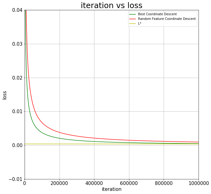
plt.figure(figsize=(10,10))
plt.plot(loss, 'g-', label='Best Coordinate Descent')
plt.plot(loss_rand, 'r-', label='Random Feature Coordinate Descent')
plt.axhline(y=L_star, color='y', label='L*')
plt.title('iteration vs loss', fontsize=25)
plt.xlabel('iteration', fontsize=15)
plt.xlim(0,1000000)
plt.ylim((-0.01,0.04))
plt.ylabel('loss', fontsize=15)
plt.xticks(fontsize=15)
plt.yticks(fontsize=15)
plt.grid()
plt.legend()

Coordinate descent loss curves for random vs best coordinate updates

Experimental Results

In this experiment I began by running an unregularized standard logistic regression solver from scikit-learn. The final cross-entropy of the logistic regression model is \(L^{*} \approx 0.0004\).

In my results, after 1.5 million updates, the coordinate descent method yields a loss \(L = 0.00047\), showing convergence to \(L^{*}\). It is important to note that both implementations of coordinate descent (random feature selection and best feature selection) converge to the loss \(L^{*}\), but at different rates.

We conclude that coordinate descent is more optimally implemented if the coordinate chosen has the largest gradient in magnitude. A clear advantage can be seen above from randomly choosing coordinates to update on.